
If you've ever written a file system traversal, built autocomplete functionality, or parsed JSON, you've worked with tree structures, whether you named them as such or not.
Trees organize hierarchical relationships. The parent nodes branch into children, leaf nodes terminate without descendants, and the whole structure descends from a single root. The concept is simple. The implementation details are where things get interesting.
Most developers encounter trees in narrow contexts such as DOM manipulation, database indexing, and compiler design, and never see the full pattern. That's a problem, because trees represent nested dependencies, enforce ordering constraints, and enable efficient traversal when relationships matter more than raw lookup speed. Understanding where trees outperform arrays, graphs, or hash tables means knowing when to reach for them instinctively, not after three failed approaches.
Let’s understand the types of trees in data structure in detail
Tree terminology
Tree data structures use specific terminology to describe node relationships, traversal patterns, and structural properties. Understanding these terms is essential for implementing search algorithms, file systems, parsing logic, and hierarchical data models correctly.
Node relationship examples
50 <- Root (depth 0, height 3)
/ \
30 70 <- Level 1 (depth 1, height 2)
/ \ \
20 40 80 <- Level 2 (depth 2, height 1)
/
10 <- Leaf (depth 3, height 0)
In this tree:
- 50 is the root with two children (30 and 70)
- 30 and 70 are siblings (same parent)
- 20 and 40 are siblings; 80 is not their sibling (different parent)
- 20, 40, and 80 are at the same level but only 20 and 40 are siblings
- 10 is a leaf node with no children
- The height of node 50 is 3 (longest path to a leaf: 50→30→20→10)
- The height of node 70 is 1 (longest path: 70→80)
- The depth of node 20 is 2 (path length from root: 50→30→20)
- Ancestors of node 10: 20, 30, 50
- Descendants of node 30: 20, 40, 10
Binary Search Trees (BST)
A Binary Search Tree extends the basic binary tree structure with an ordering constraint that enables efficient search operations. The defining property: for every node, all values in the left subtree are less than the node's value, and all values in the right subtree are greater than or equal to it. This ordering property enables search operations to eliminate half the remaining tree at each step, producing O(log n) average-case performance for balanced trees.
The power of this constraint becomes clear when searching for values. Given a tree with one million nodes that's perfectly balanced, finding any value requires at most log₂(1,000,000) ≈ 20 comparisons. Each comparison eliminates half the remaining possibilities. Compare this to searching an unsorted array, which requires examining up to one million elements. The logarithmic behavior scales remarkably well: a billion nodes requires only about 30 comparisons.
However, this O(log n) complexity carries an important caveat: it assumes the tree remains balanced. When values arrive in sorted order, the BST degenerates into a linked list where each node has only one child. This destroys the performance advantage, degrading search time from O(log n) to O(n). This is why production systems use self-balancing trees like AVL or red-black trees that maintain O(log n) guarantees regardless of insertion order. The additional rotation logic is a small price for guaranteed performance, and the absence of self-balancing is why plain BSTs rarely appear in production code outside of educational contexts.
AI-generated BST implementations frequently contain subtle bugs that pass basic tests but fail on edge cases. The most common failure involves duplicate value handling, where models write comparison logic like if value < node.value followed by else if value > node.value, completely ignoring the case where values are equal. This silently loses data. Another frequent error involves parent pointer maintenance in doubly-linked tree structures, where new nodes get inserted without updating their parent reference, corrupting tree traversal operations that depend on bidirectional navigation.
Example BST:
50
/ \
30 70
/ \ \
20 40 80
BST property verification:
- Left subtree of 50: {20, 30, 40} all < 50 ✓
- Right subtree of 50: {70, 80} all > 50 ✓
- Property holds recursively at every node ✓
Degenerate BST (sorted insertion):
Sequential insertions: 10, 20, 30, 40, 50
10
\
20
\
30
\
40
\
50
This is a linked list, not a tree.
Search for 50 requires 5 comparisons, not log₂(5) ≈ 2.3
BST Lookup Operation:
def search(node, value):
if node is None:
return False
if value == node.value:
return True
if value < node.value:
return search(node.left, value)
return search(node.right, value)
BST Insertion Operation:
def insert(node, value):
if node is None:
return Node(value)
if value < node.value:
node.left = insert(node.left, value)
elif value > node.value:
node.right = insert(node.right, value)
return node
BST In-Order Traversal (produces sorted output):
def inorder(node):
if node.left:
inorder(node.left)
print(node.value) # Visit node
if node.right:
inorder(node.right)
# Output for example tree: 20, 30, 40, 50, 70, 80
AVL Trees
AVL trees enforce a strict balance constraint: for every node, the heights of left and right subtrees differ by at most one. This guarantee prevents the degeneration problem that plagues plain BSTs. Named after inventors Georgy Adelson-Velsky and Evgenii Landis, AVL trees maintain O(log n) search time regardless of insertion order by performing rotations after insertions or deletions that would violate the balance property.
The balance factor of a node equals height(left subtree) minus height(right subtree). Valid balance factors are -1, 0, and 1. When a balance factor reaches -2 or 2, the tree performs rotations to restore balance. There are four rotation cases: left-left (right rotation), right-right (left rotation), left-right (left rotation then right rotation), and right-left (right rotation then left rotation). These rotations restructure the tree while maintaining the BST ordering property.
The strictness of AVL balance comes with a cost: more rotations during insertions and deletions compared to red-black trees. However, this strictness produces shallower trees and faster searches. For applications where searches vastly outnumber modifications, AVL trees offer better performance than red-black trees. The height of an AVL tree with n nodes is at most 1.44 × log₂(n), compared to 2 × log₂(n) for red-black trees. This difference matters at scale: for one million nodes, AVL guarantees height ≤ 29 while red-black allows height ≤ 40.
AI models frequently generate AVL rotation code with bugs that don't cause immediate failures but instead cause gradual performance degradation over many operations. The most insidious bug involves forgetting to update node heights after rotation. Heights must be recalculated bottom-up after restructuring, or subsequent balance factor calculations become incorrect, allowing the tree to drift out of balance over thousands of operations. Another common error involves updating heights in the wrong order during rotation, where the algorithm updates the new root's height before updating its children's heights, using stale height values in the calculation.
Balance factor calculation:
Balance factor = height(left subtree) - height(right subtree)
50 Balance: 2 - 1 = 1 (balanced)
/ \
30 70 Balance at 30: 1 - 0 = 1 (balanced)
/
20
After inserting 10:
50 Balance: 3 - 1 = 2 (UNBALANCED - rotation needed)
/ \
30 70 Balance at 30: 2 - 0 = 2 (UNBALANCED - rotation needed)
/
20
/
10
Right rotation on node 30:
50
/ \
20 70
/ \
10 30
Right rotation on node 50:
20
/ \
10 50
/ \
30 70
Now balanced: all balance factors are -1, 0, or 1
AVL Node Structure:
class AVLNode:
def __init__(self, data):
self.data = data
self.left = None
self.right = None
self.height = 1 # New nodes have height 1
def get_height(node):
if node is None:
return 0
return node.height
def get_balance_factor(node):
if node is None:
return 0
return get_height(node.left) - get_height(node.right)
Right Rotation:
def right_rotate(y):
x = y.left
T2 = x.right
# Perform rotation
x.right = y
y.left = T2
# Update heights (must be done bottom-up)
y.height = 1 + max(get_height(y.left), get_height(y.right))
x.height = 1 + max(get_height(x.left), get_height(x.right))
return x # New root
B-trees and B+ trees
B-trees solve a fundamental problem that binary trees cannot address efficiently: minimizing disk I/O operations. While binary trees optimize for comparisons (an in-memory operation), databases care more about reducing disk reads, because disk access is roughly 100,000 times slower than memory access. B-trees address this by allowing many keys per node and many children per node (high fanout), which reduces tree height and therefore disk reads required to find any value.
A B-tree of minimum degree t has between t-1 and 2t-1 keys per node (except the root). Each internal node with k keys has k+1 children. All leaves exist at the same depth, guaranteeing balanced performance. The critical insight: by packing hundreds of keys into a single 16 kilobyte (KB) node (matching typical disk block sizes), a three-level tree can store hundreds of millions of records. Finding any record requires exactly three disk reads regardless of dataset size, compared to potentially millions of disk reads scanning an unsorted file.
B+ trees modify the B-tree structure for database workloads. Internal nodes store only keys and child pointers (no values), allowing even more keys per node and further reducing tree height. All values reside in leaf nodes, which are linked together in a doubly-linked list. This leaf linking enables efficient range queries: find the first matching leaf via tree traversal, then follow leaf pointers to retrieve all values in the range. Without leaf linking, each result would require traversing back up the tree and down again, multiplying disk I/O.
MySQL's InnoDB storage engine stores all table data in a B+ tree where the primary key is the tree key and complete rows are the leaf values. Node size defaults to 16KB. Secondary indexes create additional B+ trees where leaf values are primary keys rather than complete rows, requiring a second lookup into the main tree to retrieve full row data. This two-lookup cost is why covering indexes (secondary indexes that include all needed columns) eliminate the second lookup and significantly improve query performance. Primary key selection fundamentally affects performance: sequential keys (auto-increment integers) cause insertions to follow the rightmost path and add new leaves only on the right, minimizing page splits and maximizing buffer pool efficiency. Random keys like Universally Unique Identifiers version 4 (UUIDv4) scatter insertions across all leaves, causing page splits throughout the tree and poor buffer pool utilization.
B+ tree structure (internal nodes vs leaf nodes):
Internal nodes (keys only, no values):
[40, 60]
/ | \
[10, 20, 30] [45, 50] [70, 80, 90]
| | |
↓ ↓ ↓
Leaf nodes (keys + values, doubly-linked):
[10:row1, 20:row2, 30:row3] ←→ [45:row4, 50:row5] ←→ [70:row6, 80:row7, 90:row8]
Range query for keys between 20 and 50:
1. Tree traversal finds first leaf containing 20
2. Follow leaf pointers right until reaching 50
3. All results retrieved with minimal disk I/O
Sequential vs random insertion impact:
Sequential (1, 2, 3, 4, ...):
- All inserts follow rightmost path
- New leaves added only on right
- Minimal page splits
- Last 5 inserts visit ~5-7 nodes
Random (UUIDv4):
- Inserts scattered across tree
- Page splits throughout tree
- Poor buffer pool efficiency
- Last 5 inserts visit ~15-25 nodes
- 3-4x more disk I/O
Why Internal Nodes Don't Store Values:
16KB node with 8-byte keys, 8-byte values, 8-byte pointers:
B-tree node capacity:
- Each entry: 8 (key) + 8 (value) + 8 (pointer) = 24 bytes
- Entries per node: 16,384 / 24 ≈ 682 entries
B+ tree internal node capacity:
- Each entry: 8 (key) + 8 (pointer) = 16 bytes
- Entries per node: 16,384 / 16 ≈ 1,024 entries
For 1 billion records:
- B-tree depth: log₆₈₂(1B) ≈ 3.4 levels → 4 disk reads
- B+ tree depth: log₁₀₂₄(1B) ≈ 3.0 levels → 3 disk reads
MySQL InnoDB Primary Key Impact:
-- BAD: Random UUID causes scattered insertions
CREATE TABLE events (
event_id UUID DEFAULT gen_random_uuid() PRIMARY KEY,
created_at TIMESTAMP,
data TEXT
);
-- GOOD: Sequential key causes rightmost-path insertions
CREATE TABLE events (
event_id BIGSERIAL PRIMARY KEY,
created_at TIMESTAMP,
data TEXT
);
-- Query performance with random vs sequential keys:
SELECT * FROM events
WHERE created_at BETWEEN '2025-01-01' AND '2025-01-31';
-- Random keys: Results scattered across many leaf nodes → 50+ disk reads
-- Sequential keys: Results in consecutive leaf nodes → 3-5 disk reads
Trie (Prefix Tree)
Tries solve a specific problem that other tree structures handle inefficiently: prefix-based string operations. Unlike BSTs where each node contains a complete value, trie nodes represent individual characters, and paths from root to nodes spell strings. This structure enables O(m) lookup time where m is string length, independent of how many strings the trie contains. A trie with one million words performs lookups just as fast as a trie with ten words, as long as the query string length remains constant.
The key advantage emerges in prefix matching scenarios. Autocomplete systems need to find all words sharing a common prefix like "inte". In a BST, this requires searching for a range of strings, examining many nodes. In a trie, navigate to the node representing "inte" (4 steps), then collect all descendants (words with this prefix). The work scales with prefix length and result count, not dictionary size. This makes tries ideal for search suggestions, spell checkers, and Internet Protocol (IP) routing tables where longest prefix matching determines packet forwarding.
Space efficiency varies dramatically based on implementation. A naive trie where each node stores an array of 26 pointers (one per letter) wastes memory when most are null. Storing children in hash maps reduces memory for sparse tries but adds hash computation overhead. Radix trees (compressed tries) merge single-child paths into nodes labeled with multi-character strings, dramatically reducing node count for words with long unique suffixes. The Linux kernel's radix tree implementation efficiently stores page cache mappings using this compression.
The most common AI-generated trie bug involves forgetting to mark word endings. Without an is_end_of_word flag, searches return false positives: searching for "cat" returns true if the trie contains "catch", because "cat" is a prefix of "catch". Another frequent error involves inefficient deletion implementations that fail to clean up unused branches. When removing "catch", if no other words share its prefix, the entire branch should be deleted to reclaim memory. AI-generated code often leaves orphaned branches that accumulate over thousands of deletions, causing memory leaks.
Trie storing: "cat", "car", "card", "dog"
Root
├─ c
│ ├─ a
│ │ ├─ t (end) → "cat"
│ │ └─ r
│ │ └─ (end) → "car"
│ │ └─ d (end) → "card"
└─ d
└─ o
└─ g (end) → "dog"
Properties:
- Shared prefixes stored once ("ca" shared by cat/car/card)
- Search time O(m) where m = string length
- Memory usage O(ALPHABET_SIZE × N × M)
where N = number of strings, M = average length
Prefix search for "ca":
1. Navigate root → c → a (2 steps)
2. Collect all descendants: "cat", "car", "card"
3. Time independent of total dictionary size
Trie Node Structure:
class TrieNode:
def __init__(self):
self.children = {} # Maps char → TrieNode
self.is_end_of_word = False
Trie Insert Operation:
def insert(root, word):
node = root
for char in word:
if char not in node.children:
node.children[char] = TrieNode()
node = node.children[char]
node.is_end_of_word = True # Critical: marks complete word
Trie Search Operation:
def search(root, word):
node = root
for char in word:
if char not in node.children:
return False
node = node.children[char]
return node.is_end_of_word # Must check end marker
# Common bug (missing end marker check):
# return True # Wrong: returns true for prefixes too
Trie Prefix Search:
def find_with_prefix(root, prefix):
node = root
# Navigate to prefix node
for char in prefix:
if char not in node.children:
return []
node = node.children[char]
# Collect all complete words from this point
results = []
collect_words(node, prefix, results)
return results
def collect_words(node, current_word, results):
if node.is_end_of_word:
results.append(current_word)
for char, child in node.children.items():
collect_words(child, current_word + char, results)
Here's a general tree node in Python:
class TreeNode:
def __init__(self, data):
self.data = data
self.children = [] # List of child nodes
def add_child(self, child_node):
self.children.append(child_node)
def is_leaf(self):
return len(self.children) == 0
When evaluating AI-generated code implementing tree structures, verify that the node class properly tracks parent-child relationships and that operations maintain the tree's structural integrity.
Why tree structures matter for AI training
Trees are the underlying representation that models manipulate when they generate code, parse documents, and construct reasoning chains. Here’s why they matter in AI training:
Code parsing and abstract syntax trees
Every programming language parses source code into an abstract syntax tree (AST) before compilation or execution. The tree represents the hierarchical structure of the code: a function contains statements, statements contain expressions, expressions contain operators and operands.
Consider this Python function:
def calculate_total(items):
total = 0
for item in items:
if item.price > 0:
total += item.price
return total
The AST for this code has the function definition as root, with child nodes for the assignment, for-loop, and return statement. The for-loop node has children for the iterator and the if-statement. The if-statement has children for the condition and the body.
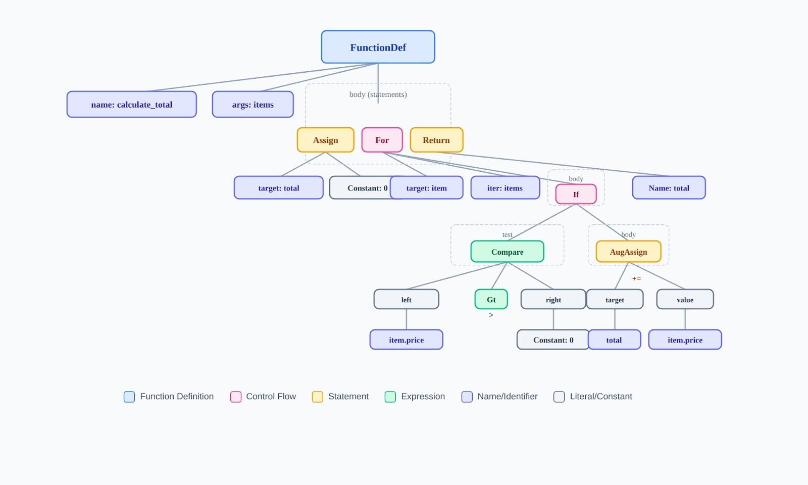
What this means for evaluation: When a model generates code with a syntax error, the AST is malformed. When code has structural problems (excessive nesting, unclear control flow), the AST reveals why — even if the code technically runs.
Document structure and the DOM
HTML documents are trees. The <html> tag is the root. <head> and <body> are its children. Every nested tag creates another level in the tree.
<html> <!-- Root -->
<head> <!-- Child of html -->
<title>Page</title> <!-- Child of head, leaf node -->
</head>
<body> <!-- Child of html, sibling of head -->
<div> <!-- Child of body -->
<p>Text</p> <!-- Child of div, leaf node -->
</div>
</body>
</html>
When evaluating AI-generated HTML, a <div> closed in the wrong place restructures the entire subtree. Accessibility issues often stem from tree-structure problems: screen readers navigate the DOM, so malformed hierarchies create unusable pages.
Decision and reasoning hierarchies
When models reason through multi-step problems, they construct implicit decision trees. Each choice branches into consequences. The structure of this tree determines whether the logic is sound.
Common reasoning tree failures to catch:
Different tree types have different constraints and use cases. Understanding these distinctions helps you evaluate whether AI-generated solutions use appropriate structures.
Tree traversal algorithms
Traversal determines the order in which you visit nodes. The choice must match the problem; using the wrong traversal produces incorrect results.
Depth-first traversals
def preorder(node):
"""Visit root, then left, then right"""
if node is None:
return
print(node.data) # Process node first
preorder(node.left)
preorder(node.right)
def inorder(node):
"""Visit left, then root, then right"""
if node is None:
return
inorder(node.left)
print(node.data) # Process node in middle
inorder(node.right)
def postorder(node):
"""Visit left, then right, then root"""
if node is None:
return
postorder(node.left)
postorder(node.right)
print(node.data) # Process node last
When to use each traversal:
Deleting nodes safely, postfix expression
Breadth-first traversal
BFS explores all nodes at the current level before moving deeper. It requires a queue.
from collections import deque
def bfs(root):
if root is None:
return
queue = deque([root])
while queue:
node = queue.popleft() # Remove from front
print(node.data)
if node.left:
queue.append(node.left) # Add to back
if node.right:
queue.append(node.right) # Add to back
Critical evaluation point: AI-generated BFS code that uses a stack instead of a queue is wrong. It will visit all nodes but in DFS order, not level order. This is a common bug.
Data Structure
Traversal Type
Order
Queue (FIFO)
BFS
Level by level
Stack (LIFO)
DFS
Branch by branch
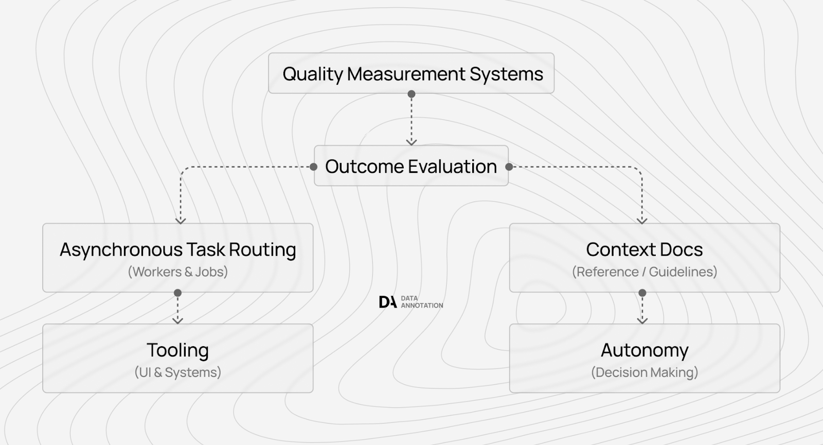
Contribute to frontier AI development
If you understand data structures at this level ; not memorized interview answers, but actual structural reasoning, you have the foundation for expert AI training work.
Coding projects involve evaluating AI-generated solutions across Python, JavaScript, C++, Java, and other languages. You assess correctness, efficiency, and maintainability. You catch the structural bugs that determine whether models improve. Your expertise directly shapes how frontier AI systems develop.
Getting started: visit the DataAnnotation application page and complete the Coding Starter Assessment. This isn't a resume screen but rather, a demonstration of whether you can actually do the work. The assessment typically takes one to two hours.
No signup fees. DataAnnotation stays selective to maintain quality standards. You can only take the Starter Assessment once, so read the instructions carefully and review before submitting.
Apply to DataAnnotation if you have the technical depth to evaluate code at a structural level and you want work that advances frontier AI capabilities.
.jpeg)